Users of the R programming language can generate documents that include text, code, and visuals using the RMarkdown tool. By combining your R code with text, equations, and graphics, you can quickly produce reproducible reports, presentations, and even web pages with RMarkdown.
RMarkdown documents may blend text, code, and output thanks to its straightforward markup language. The papers can be transformed from plain text to a number of other forms, such as HTML, PDF, Microsoft Word, and more.
The ability to create entirely reproducible documents is one of the key advantages of utilising RMarkdown. By running the same code and producing the same findings, anyone can duplicate your analysis. RMarkdown can also speed up your productivity by giving you the freedom to concentrate on the content of your manuscript rather than the formatting.
Simply begin with a plain text file with the .Rmd suffix to create an RMarkdown document, and then add your code and output using R code chunks. Markdown syntax can be used to format text, add headings, lists, and more. Once you have finished your document, you can use the knit function in RStudio to convert it to the desired format.
Contents
How to use rmarkdown
You must have R and RStudio installed on your computer in order to use RMarkdown. To produce an RMarkdown document, complete the following steps after installing R and RStudio:
- Click “File” > “New File” > “R Markdown” in RStudio.
- Give your document a title, choose a place to save it in, and choose the output format you desire (such as HTML, PDF, Word, etc.) in the “New R Markdown” dialogue box.
- To start a new RMarkdown document, click “OK”.
To assist you in getting started, your new RMarkdown document will open in the RStudio editor with some pre-populated text and code.
You can combine Markdown syntax and R code chunks to add content to your RMarkdown page. R code chunks are used to run R code and display the results in your document, while Markdown syntax is used to format text, generate headings, lists, and more.
Rmarkdown is basically characterized into two different sections:
- YAML
- Body
YAML
The data serialisation language YAML (short for “YAML Ain’t Markup Language”) is frequently used in R Markdown documents to express metadata and document settings. The title, author, date, output format, and other settings of a R Markdown document are specified using YAML in the “front matter” section.
Here is an illustration of a YAML header that could appear at the start of a R Markdown document:
---
title: "My R Markdown Document"
author: "Jane Doe"
date: "2023-03-09"
output:
  html_document:
    theme: cosmo
    toc: true
    toc_depth: 2
---
The YAML header in this instance begins and ends with three dashes (—). The header has numerous lines of key-value pairs, with a colon separating the key from the value in each pair (:).
- The metadata fields
title,author, anddateinclude information on the document’s title, author, and date. outputis a top-level key that describes the document’s output format. In this instance, the html document format is being used, and the output is an HTML file.- Options specific to the html document
outputformat include theme, toc, and toc depth. We’re using the Bootstrap theme cosmo in this example, and we’re also including a table of contents (toc) with a depth of 2.
The appearance and behaviour of the produced output can be affected by a number of options that you can specify by including a YAML header in your R Markdown text. See the R Markdown documentation for a complete list of the parameters that can be used in the YAML header.
Body
The primary content of your document, which may include text, code snippets, inline expressions, tables, photos, and other components, is contained in the body of a R Markdown document. The body of a R Markdown document is written using a combination of code chunks written in the language of your choosing and Markdown syntax (e.g., R, Python, etc.).
Here is an illustration of a straightforward R Markdown document with some body content.
Add headings
In R Markdown, headings can be added by using the hash symbol #, a space, and then the heading’s text.
In R Markdown, there are six levels of headings, with # denoting the top-level (biggest) heading and ###### denoting the bottom-level (smallest). Here’s an illustration:
# Top-level heading
## Second-level heading
### Third-level heading
#### Fourth-level heading
##### Fifth-level heading
###### Sixth-level heading

A first-level heading or a second-level heading can also be made by placing === or —- under a line of text, respectively:
Although there are several syntaxes available in R Markdown for constructing headings, such as dashes or equal signs, the hash symbol syntax is the most popular and flexible.
Adding bullets and numbered lists
Unordered list
Use the – or * character followed by a space at the beginning of each line to create an unordered list in R Markdown. This will create an unordered list with bullets.
- Item 1
- Item 2
- Item 3

Numbered list
Use the digits 1., 2., 3., etc. followed by a space at the start of each line to generate an ordered list in R Markdown. This will create an ordered list with numbers.
1. Item 1
2. Item 2
3. Item 3

Nested lists
By indenting lists, you can nest them as well. This will create a nested bulleted list:
- Item 1
  - Subitem 1
  - Subitem 2
- Item 2
  - Subitem 1
  - Subitem 2
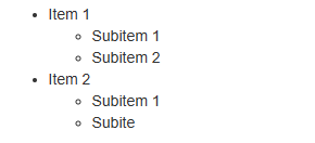
Moreover, nested lists can be made by indenting elements with tabs or spaces. For instance:
1. Item 1
   1. Subitem 1
   2. Subitem 2
2. Item 2
   1. Subitem 1
   2. Subitem 2
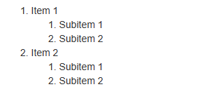
Adding codes
Use the code chunk functionality to include code in a R Markdown text. You can embed executable code in your document that can be examined and shown using code chunks. To add code chunks to your R Markdown document, follow these steps:
- Start a new code chunk by typing three backticks (` ` `) followed by the letter “r“. Then press enter to start a new line and end with three backticks.
```{r}# This is an R code chunk```
- Insert your R code enclosed with three backticks will create the output from the code. Here is an illustration:
```{r}
2 + 2
```
# 4
Code snippets are by default concealed in the document’s final output. You can include the option echo = TRUE in the code chunk header, like in the following, to display both the code and its output:
Adding equations
- Start a new line and enclose the equation in dollar signs. For example, to display the equation “y = a + bx”, type:
- To include more complex equations, you can use LaTeX syntax. For example, to display the equation for the normal distribution, type:
- Bold text: To bold text, surround the text with two asterisks (**). For example,
**this text is bold**will display as this text is bold. - Italic text: To italicize text, surround the text with one asterisk (*). For example,
*this text is italicized*will display as this text is italicized. - Bold and italic text: To make text both bold and italic, surround the text with three asterisks (***). For example,
***this text is bold and italic***will display as this text is bold and italic. - Underline text: To underline text, surround the text with two square brackets ([]) and then in curly braces type {.underline}. For example, [
this text is underlined]{.underline} will display as this text is underlined. - Save the image file in the same directory as your RMarkdown document, or in a subdirectory.
- In your RMarkdown document, use the following syntax to insert the image:
Use LaTeX syntax to include an equation in a R Markdown page. R Markdown equations are typically added using the typesetting language LaTeX, which is typically used for technical and scientific writings.
Display equation
To display an equation in RMarkdown, you can use the $$...$$ syntax.
$y = a + bx$$$y = a + bx$$
$
G%=frac{sum n_i}{N}
$
$$G%=frac{sum n_i}{N}$$
Inline equation
To include an inline equation in RMarkdown, you can use the $...$ syntax. Here’s an example:
The formula for the area of a circle is given by $A=pi r^2$,
where $r$ is the radius.
The output will look like this:
The formula for the area of a circle is given by \(A=pi r^2\), where \(r\) is the radius.
The equations in your R Markdown document will be typeset using LaTeX syntax when it is rendered. Several resources, such as the LaTeX documentation and cheat sheets, are available online if you are unfamiliar with the syntax of LaTeX.
Emphasizing text
In RMarkdown, you can emphasize text in several ways:
Adding images
You can add images to your RMarkdown document using the following steps:
You can also specify the width and height of the image by adding “width” and “height” attributes to the image tag, like this:
{ width=50% }
You can also add images by using include_graphics() function from knitr package in rmarkdown chunk. The include_graphics() function is a part of knitr package and insert graphics into your document. You can use the fig.width and fig.height chunk option to specify the width of the output graphics for a particular code chunk. This option sets the width of the graphics device in inches.
You can use the below code to add graphics to your rmarkdown document:
```{r, fig.width=6, fig.height=6, dpi = 300}
knitr::include_graphics(path = "path/to/image.png", dpi = 300)
```
Getting the output
The “Knit” button in the RStudio editor or the keyboard shortcut “Ctrl + Shift + K” (Windows) or “Cmd + Shift + K” can be used to knit your RMarkdown document (Mac). The format you choose when you produced the document will be used by RStudio to build the output document.
That’s a brief introduction to using RMarkdown. I strongly advise you to look through the RMarkdown documentation to understand more about the many additional features and choices available.

